

Figures and tables
Tables and figures are examples of entities that 'float'. They generally form too large an entity to be conveniently placed just anywhere on a page. Instead LaTeX waits so that it can put them in a convenient place: the top of a page, the bottom of a page, or on a page by itself.
Let LaTeX float tables and figures, do not try to insist that you know better.
From research by Colin Wheildon: "Seventy-seven
percent [of readers] said articles in which body type jumped
over an illustration ..., contrary to the natural flow of
reading, annoyed them. The natural expectation was that once
a barrier such as an illustration ... was reached, the
article would be continued at the head of the next leg of
type."
Tables
To request LaTeX to include a table use the table environment:
\begin{table}
 \caption{...}
 \label{...}
 ...
 instructions for typesetting the table
 (usually tabular within a center environment,
 or array within a displaymath environment)
 ...
\end{table}
See the table of fractal dimensions at the end of Src/fractals31.tex. In the first run through, LaTeX cannot find room on page 5 for the table, and so places it on page 6 by itself. In the second run, the Table of Contents has pushed more material into the document, and now the table is placed at the top of the page.
- If your data is mostly text with some mathematics, then typeset in the tabular environment within a center environment. Typeset mathematical entries within $...$, or better is \(...\).
- If your data is mostly mathematics, even if simply numbers, then typeset in the array environment within a displaymath environment (the arguments of the array environment are the same as those of the tabular environment). Typeset the textual entries within \text{...}, or if relatively long then \parbox{width}{\raggedright ...}.
My table has few drawn lines: this is best practice. Let the grid structure of a table work for you without the distraction of zillions of horizontal and vertical lines. Use lines sparingly.
For tables of numbers, only report as few as digits as possible to convey the message.
For example, many authors report "errors" to four significant digits, and almost always there is no justifiable reason. As copyeditor I truncate to two digits, but really one significant digit is almost always sufficient for errors. Do not report more.
From James Hartley, Academic writing and
publishing: "round off the numbers so that
readers can make meaningful comparisons more
easily"
One may include a List of Tables in the document with the command \listoftables.
Figures
See video discussion 42
Just as for tables, somewhere near where you need the figure, usually at the start of the first paragraph that discusses the figure, include the figure environment
\begin{figure}\centering
 ... graphic LaTeX code ...
 \caption{...}
 \label{...}
\end{figure}
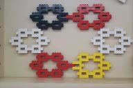
The example
Src/fractals34.tex shows how to
\usepackage{graphicx} in order to include a figure
of the lego fractal jpeg picture Share/sflower.jpg.
In twocolumn documents a figure is usually placed within one column, but the figure* environment instead spreads a figure over both columns.
Of course, mostly scientific or engineering graphics are not pictures, but plots. There are several good possibilities for the LaTeX code that includes a plotted graph, and analogous possibilities with other computing languages:
- draw graph in Matlab, Octave, R, etc, export to pdf, include in the LaTeX;
- draw graph in Matlab or Octave, export to LaTeX code, input the code into your source;
- or code 'pgfplots' commands yourself directly into your LaTeX source.
One may include a List of Figures in the document with the command \listoffigures.
One could alternatively put the \caption{} and \label{} above the graphic, as then hyperlinks to the figure will move to a better position. We are already used to titles being above graphics, and I know of no research finding that captions above graphics hinder comprehension by a reader.
Small graphics
Place small graphics (or indeed anything) into the margin with the command \marginpar{...}, and you may need to change its width via say
\setlength{\marginparwidth}{6em}
For example, download my thumbnail
picture and include it in the margin with
\marginpar{\includegraphics{tonyroberts}}
For best results with marginpars include the preamble
\usepackage{marginfix}.
Alternatively, the wrapfig package empowers us to wrap text around a graph, or indeed around any rectangular area of typeset material, but use only with care, and also with the needspace package.
Avoid animations, movies and VR-3D
It is possible to include animations, movies, and interactive 'virtual reality' 3D graphics within pdf documents via LaTeX (see examples). However, many pdf readers do not support them, and almost no journal supports their inclusion. So avoid :(Stunning graphs with pgfplots
See video discussion 43Obtain stunning quality graphics within LaTeX using the pgfplots package by invoking in the preamble
\usepackage{pgfplots}
\pgfplotsset{compat=newest}
To get started, see this
introduction, then see a host of examples at PGFPlots.net
The cost of these beautiful pgfplots is a major slow down of LaTeX as it draws the graphs (although one can 'externalize' and recover the speed).
Alternatively, draw the graph in Matlab or Octave, then export to pgfplots-LaTeX code with matlab2tikz() function. I recommend invoking with something like
cleanfigure;
matlab2tikz('filename.tex'...
,'showInfo',false,'noSize',true...
,'parseStrings',false,'showWarnings',false ...
,'extraCode','\tikzsetnextfilename{xxxx}' ...
,'extraAxisOptions',string ...
)
Currently (2020) there is a bug in matlab2tikz().
If you get unwanted legends appearing in your plots, then
edit line 1064 of matlab2tikz.m by replacing
"legendhandle = legend(axisHandle);" with
"legendhandle = axisHandle.Legend;" This
replacement should omit the unwanted legends for you.
Graphs via postscript within pdf
See video discussion 44The usual way to include a figure in LaTeX is, as follows, to draw the graph in Matlab, Octave, R, etc, export to postscript, convert to pdf, include in the LaTeX. But by now in the 2020s most software and journals have caught up to pdf being the preferred format, so nowadays one rarely needs the postscript.
Do not export to bit-image formats such as .png, .gif, .tiff, or .jpg Remember that pdf-format is just a wrapper around almost any sort of information. It is all too easy, and fatal, to end up with a pdf-file containing a bit-image graphic. Avoid doing so.
- Create a vector-graphic pdf file of the drawing
from whatever application is being used to generate the
figure. For example,
Src/cantor.m and
Src/koch.m are Matlab programs that create
postscript graphs in files
Src/cantor.pdf and
Src/koch.pdf. Obtain these in Matlab post-2020 via
the command
exportgraphics(gcf,'filename.pdf' ...
    ,'ContentType','vector')
or pre-2020 prefer the following command and convert to pdf afterwardsprint('-depsc','filename')If the graphic is photograph-like, either because it is a photograph or because it is a surface plot with smooth graduations, then create as the non-vector bit-image format of jpeg rather than pdf.
- Then place in the preamble the commands
\usepackage{graphicx} - Somewhere near where you want the figure, include the
figure environment
\begin{figure}\centering
 \includegraphics{...}
 \caption{...}
 \label{...}
\end{figure}
where the argument of the \includegraphics command is the filename (without the extension). - Or use this to scale the picture up/down, but only a
little,
\begin{figure}\centering
 \includegraphics[scale=0.9]
     {...}
 \caption{...}
 \label{...}
\end{figure}
See the two figures in Src/fractals32.tex
The scale=0.9 scales the figure to 90% of the size of the drawn graphic: scaling between 0.9--1.1 is fine; scaling between 0.8--1.2 is probably OK; but avoid any more drastic scalings.
I strongly urge you to generate the graphics at about the same size as they are to appear.
This sizing is so that the title, label and legend information is readable and the line thicknesses are credible (avoid grotesque scaling such as this), or this even worse example.
- Most journals, and good dissertation styles, typeset
to a text-width of about 14cm. Consequently,
- a single graph must be no more than 140mm wide;
- two side-by-side graphs no more than 70mm wide each;
- and so on.
- For two column journals or proceedings, a single graph, to fit into a single column, must be no more than about 90mm wide.
Unfortunately, much software, such as Matlab, by default generate graphics that are far too big! You must override. For three examples:
- Src/koch.m uses Matlab's subplot(3,3,n) for n=1,2,4,5 in order to generate a four-part graphic close to the correct size of the width of body text;
- Src/cantor.m uses Matlab's set(gca,'position',[.2 .2 .6 .6]) before the export-graphics in order to set the size close to the width of body text;
- for Maple, an internet search suggests that before
you issue a plot command, invoke
plotsetup(postscript,
plotoutput=`image.ps`,plotoptions=
`color,portrait,height=300,width=300`);
set(gca,'position',[.2 .2 r r])
exportgraphics(gcf,'filename.pdf' ...
    ,'ContentType','vector')
This ensures you get great quality vector graphics at close
to the size needed for including into your LaTeX. Do
similarly for other software.
Always code into a script the commands that generate a graphic.
- Even though in exploring how to generate a graphic you may use a graphical user interface, ultimately reproducible research requires that you must codify the process, including codifying the `export' command that actually outputs the tex/pdf/jpeg file.
-
Ensure your graphics are traceable back to the source file
that generated them. I recommend prefixing the name of the
script file to the name of the graphic file. That is, if a
script named abc.* generates a graph on topic
xyz, then name the graphic file abcxyz.*
For example, if using Matlab/Octave, then invoke the function
mfilename as in
exportgraphics(gcf,[mfilename 'xyz.pdf'])
ormatlab2tikz([mfilename 'xyz.tex'], ...