Chapter 3 solutions to odd numbered exercises

• Exercise 3.1

  1. Color is categorical with no meaningful order in this context.
  2. Orders is a discrete non-negative integer.
  3. Cost is continuous. (It is not helpful to consider the cost as a discrete number of cents, and we can think of an underlying continuous cost rounded to the nearest cent.)
  4. Resistance is continuous
  5. Temperature is continuous
  6. Safety assessment is categorical, ordered by level of achievement. An ordered categorical variable is referred to as an ordinal variable.
  7. Number of employees on leave each day is non-negative discrete, but it might be considered as continuous in a large organisation.
  8. Number of employees in cars is a discrete positive integer.
  9. Gain is continuous.
  10. The number of different models is a discrete positive integer.

Top

• Exercise 3.3

  1. \(g(a) = \sum (x_i - a)^2\)
     \(dg/da = \sum -2(x_i - a)\)
     A necessary condition for a minimum is \(dg/da = 0\)
     \(dg/da = 0\) implies \(a = \sum x_i/n = \overline{x}\)
  2. \((n-1) \times s^{2} = \sum (x_i - \overline{x})^{2} = \sum (x_i - \mu)^{2} = n \times \hat{\sigma}^{2}\)
     A rationale for using \((n-1)\) in the denominator of \(s^{2}\) is that it compensates for the numerator being, almost certainly, slightly less than the sum of squared deviations from the population mean.

Top

• Exercise 3.5

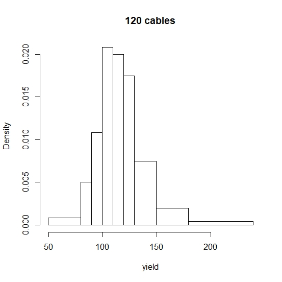
  The low frequency of \(2\) in the \(120-129\) bin is striking. We are told that there are \(120\) sample lengths, so the sum of the frequencies should be \(120\). The sum of the given frequencies is \(101\), so the \(2\) is a transcription error and should be \(21\). See supplementary exercise \(S3.1\) for the solution if the \(2\) is supposed to be correct and the sample size is \(101\).
  1. The class intervals are of different lengths so the vertical scale needs to be relative frequency density. Also, we need to use relative frequency density for the area under the histogram to equal \(1\). The calculations for the relative frequency densities (rfd) are shown below. The bins have been defined so that, for example, the \(100\) to \(109\) bin includes yields between \(99.50\) recurring and \(109.50\) recurring. The width is \(10\) and the mid-point is \(104.5\). If the yield measurements are rounded to the nearest integer this bin includes yields from \(100\) up to \(109\).

     > #bin mid points (bm), bin widths (bw) and frequencies (freq)
     > bm=c(64.5,84.5,94.5,104.5,114.5,124.5,139.5,164.5,209.5)
     > bw=c(30,10,10,10,10,10,20,30,60)
     > freq=c(3,6,13,25,24,21,18,7,3)
     > n=sum(freq)
     > rf=freq/n
     > rfd=round(rf/bw,4)
     > print(cbind(bm,rfd))
     bm rfd
     [1,] 64.5 0.0008
     [2,] 84.5 0.0050
     [3,] 94.5 0.0108
     [4,] 104.5 0.0208
     [5,] 114.5 0.0200
     [6,] 124.5 0.0175
     [7,] 139.5 0.0075
     [8,] 164.5 0.0019
     [9,] 209.5 0.0004
     

     The following R code draws the histogram. Notice that assuming all the data coincide with mid-points of the bin will give a correct histogram.

     > #histogram
     > #cut points for bins (cp)
     cp=c(49.5,79.5,89.5,99.5,109.5,119.5,129.5,149.5,179.5,239.5)
     > x=rep(bm,freq)
     > hist(x,breaks=cp,xlab="yield",main="120 cables")
     

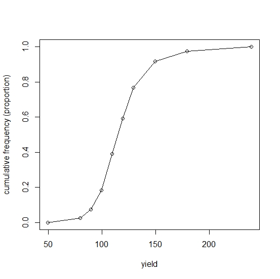
  2. The following R code plots the cumulative frequency polygon.

     #cumulative frequency polygon
     cfprop=cumsum(freq)/120
     cf=c(0,cfprop)
     plot(cp,cf,xlab="yield",ylab="cumulative frequency (proportion)")
     lines(cp,cf, type = "l")
     

  3. median
         \(0.5\) corresponds to \(60/120\)
         \(47\) yields less than or equal to \(109.5\) and \(71\) less than or equal to \(119.5\)
         \(109.5 + (13/24) \times (119.5 - 109.5)\)
         [1] 114.9167
         An approximate median is \(115\) as can be checked from the cumulative frequency polygon
     LQ
         \(0.25\) corresponds to \(30/120\)
         \(22\) yields less than or equal to \(99.5\) and \(45\) less than or equal to \(109.5\)
         \(99.5 + (8/23) \times (109.5 - 99.5) = 102.9783\)
         An approximate LQ is \(103\) as can be checked from the cumulative frequency polygon
     UQ
         \(0.75\) corresponds to \(90/120\)
         \(71\) less than or equal to \(119.5\) and \(92\) less than or equal to \(129.5\)
         \(119.5 + (19/21) \times (129.5 - 119.5) = 128.5476\)
         An approximate UQ is \(129\) as can be checked from the cumulative frequency polygon.
     The IQR is \(128.5 - 114.9\) which is approximately \(15\)
     
     NOTE Using bin cut = points of \(50, 60, 90\) etc will make negligible difference to the graphs and increase the approximate median and quartiles by \(0.5\) which is also slight.

Top

(To be continued)