The weighted estimate of the population mean is \(27.050\)
The weighted estimate of the population variance is \(0.001068132\)
The weighted estimate of the population standard deviation is \(0.033\)
The estimated proportion outside the specification is \(0.126\).
[The proportion outside specification is too high. Can the process standard
deviation be reduced by improving procedures? Can the specification be relaxed?
If neither apply is it worth the supplier investing in machinery with higher
precision?]
Exercise 6.3
\(c = \rho \times\sigma_{X} \times \sigma_{Y}\)
The mean of \(X + a\) is \(\mu_{X} + a\) and similarly for \(Y\)
and therefore \(X + a - (\mu_{X} +a) = X - \mu_{X}\) and similarly for
\(Y\) and the covariance will be unchanged.
We can choose \(a = -\mu_{X}\) and \(b = -\mu_{Y}\), and the covariance of
mean adjusted variables is identical to the covariance of the original variables. The practical
consequence is that we can assume variables have a mean of \(0\), without loss of generality, when proving
results about covariances.
\(\overline{Y} = \sum \dfrac{Y_{i}}{n}\).
We can assume without loss of generality that the mean of \(X\) and the mean of \(Y\) is \(0\).
Then the covariance of \(\overline{X}\) and \(\overline{Y}\) is
\(E\left[\sum X_i \times \sum \dfrac{Y_{i}}{n^2} \right] = \dfrac{nc}{n^2} = \dfrac{c}{n}\) since \(X_{i}\) and
\(Y_{j}\) are independent unless \(i = j\).
The correlation between \(\overline{X}\) and \(\overline{Y}\) is
\(\dfrac{\frac{c}{n}}{\frac{\sigma_{X}}{\sqrt{n}}} \times \frac{\sigma_{Y}}{\sqrt{n}} = \rho\)
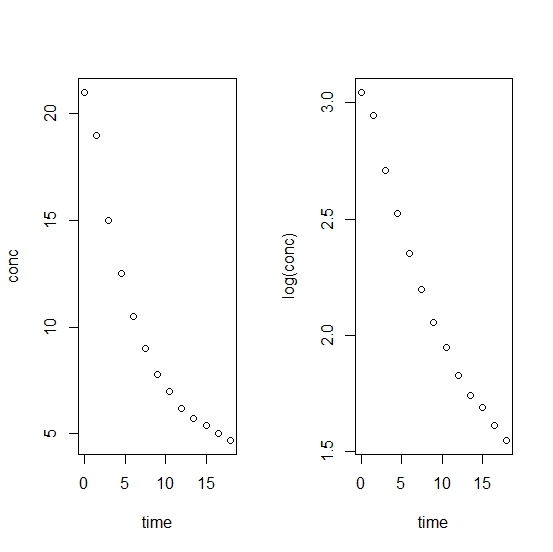
The correlation is \(-0.933\). The concentration decreases with time, and there is a corresponding
high, in absolute value, negative correlation. However, the plot shows a distinct tendency for
the decrease in concentration over time to reduce in absolute terms.
If we plot the logarithm of concentration against time the relationship is closer to linear and the correlation is
\(-0.983\).
It is likely that taking \(\log{(conc-L)}\) where \(L\) is some lower limit would give an even closer
linear relationship (for example, taking \(L=4\) gives a correlation of \(-0.9989983\)).
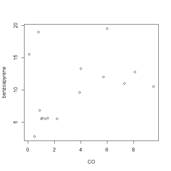
The correlation is positive but only slight. There is a discernible tendency for
benzoapyrene to increase as CO increases, but there is considerable scatter about a linear relationship.
Exercise 6.9
\(F(x,y) = \displaystyle \int_0^y \int_0^x (u+v) du dv\)
\(\hspace{14mm}= \displaystyle \int_0^y \left[\frac{u^2}{2} + u v \right]_0^x dv\)
\(\hspace{14mm}= \displaystyle \int_0^y \left(\frac{x^2}{2} + x v \right)dv\)
\(\hspace{14mm}= \displaystyle \left[v \frac{x^2}{2} + x \frac{xv^2}{2} \right]_0^y\)
\(\hspace{14mm}= \displaystyle \frac{1}{2} \left(x^2y + xy^2\right), \quad 0 \le x,y, \le 1\)
\(f(x|y) = \displaystyle\frac{f(x,y)}{f(y)}\)
\(\hspace{12mm}= \displaystyle\frac{x + y}{\frac{1}{2} + y}, \quad 0 \le x \le 1 \mbox{ for } 0 \le y \le 1\)
Check by finding \(F(x|y) = \displaystyle\frac{\frac{x^2}{2} +xy}{\frac{1}{2} + y}\) and verifying that
\(F(0|y) = 0\) and \(F(1|y) = 1\)
Exercise 6.15
Let \(X\) be the clearance: hole diameter - rivet diameter
The random selection justifies an assumption that hole and rivet diameters are independent.
Mean of \(X\) is \(2.35 - 2.30 = 0.05\)
Variance of \(X\) is \(0.1^2 + 0.05^2 = 0.0125\)
(covariance is \(O\) since hole and rivet diameters are independent)
Assume that the rivet will fit if the clearance is positive.
> mu=2.35-2.30
> v=0.1^2+0.05^2
> v
[1] 0.0125
> sig=sqrt(v)
> sig
[1] 0.1118034
> 1-pnorm(0,mu,sig)
[1] 0.6726396
The probability of a fit is \(0.673\). This is far too low for sustainable manufacturing.
Exercise 6.17
\(T\) has mean \(100 + 100 + 100 = 300\)
\(T\) has variance \(30^2 + 30^2 + 30^2 = 2700\)
The standard deviation is the quare root of the variance \(51.96\)
The distribution is normal because \(T\) is a linear combination of normal random variables.
We need the probability that \(T\) exceeds \(200\)
The probability that three batteries will suffice is \(0.973\).
Let \(M\) be the mission length. We need the distribution of \(T - M\), which is normal
with mean \(300 - 200 = 100\), and given the independence of \(T\) and \(M\), standard
deviation \(= \sqrt{2700+50^2}\).
We need the probability that \(T - M\) is positive.
The probability that three batteries will suffice is now \(0.917\).
Notice that it is reduced because of the uncertainty about the duration of the mission.
Exercise 6.19
\(W\) has mean \(5 \times 720 = 3600\) and, given independence, variance
\(5 \times 75^2 = 28125\).
It follows that the stadard deviation is \(167.7\)
The mean of \(W\) is \(5 \times 720 = 3600\)
The variance of \(W\) is the sum of the variances for the \(5\) days plus twice the covariances between
\(Day1\) and \(Day2\), ... , \(Day1\) and \(Day5\), and \(Day2\) and \(Day3\), ... ,\(Day5\),
... , \(Day4\) and \(Day5\):
\(5 \times 75^2 + 2 \times 75^2 \times (0.8 + 0.8^2 + 0.8^3
+ 0.8^4 + 0.8 + 0.8^2 + 0.8^3 + 0.8 + 0.8^2 + 0.8) = 101853\)
The standard deviation is \(319.1\)
\(mean = \sum_{i=1}^n a_{i} \mu_{i}\)
The variance is neatly expressed as a double sum
\(variance = \sum_{i=1}^n \sum_{j=1}^n a_{i} a_{j} g_{ij}\),
where \(g_{ii}\) is the variance of \(X_{i}\). Check it gives the answer in b. when \(n = 3\).
The standard deviation is the square root of the variance.