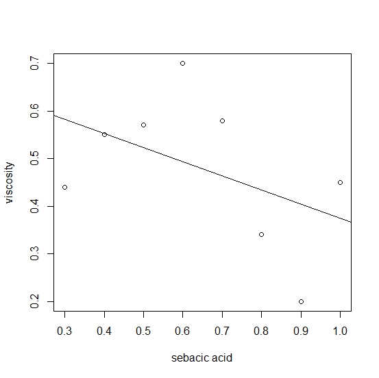
Random variation about a straight line with a negative slope appears plausible.
> m1=lm(y~x)
> summary(m1)
Call:
lm(formula = y ~ x)
Residuals:
Min 1Q Median 3Q Max
-0.20464 -0.10634 0.02196 0.08527 0.20643
Coefficients:
Estimate Std. Error t value Pr(>|t|)
(Intercept) 0.6714 0.1595 4.209 0.00563 **
x -0.2964 0.2314 -1.281 0.24754
---
Signif. codes: 0 *** 0.001** 0.01 * 0.05 . 0.1 1
Residual standard error: 0.15 on 6 degrees of freedom
Multiple R-squared: 0.2147, Adjusted R-squared: 0.08382
F-statistic: 1.64 on 1 and 6 DF, p-value: 0.2475
The estimate of the slope is \(-0.296\) but the sample size is small and its
estimated standard error is \(0.231\). The associated p-value is \(0.248\), so it is not
statistically significantly different from \(0\) at the \(0.10\) level of significance.
There is not sufficient evidence to reject a hypothesis that the slope is \(0\) at the \(0.10\) level of significance.
[If we increased the sample size the estimated standard error of the slope (coefficient
of sebacic acid) will reduce and we might have evidence of a linear relationship. However,
there is no reason to expect that the ratio of the estimated standard deviation of the errors
to the standard deviation of viscosity will decrease. It follows that even a statistically
significant regression is unlikely to be useful for controlling or predicting viscosity.]